Why Steering Works – The Theory Beneath X Engineering for AI Agents
July 26, 2026
An agent run is stochastic gradient descent over solution space, and steering is how the true objective enters the loop. An optimization view and a Bayesian view that ground the industry ladder — prompt, context, harness, loop engineering — in foundation theory, and explain when a big model steering a small one beats distillation, and when it does not.
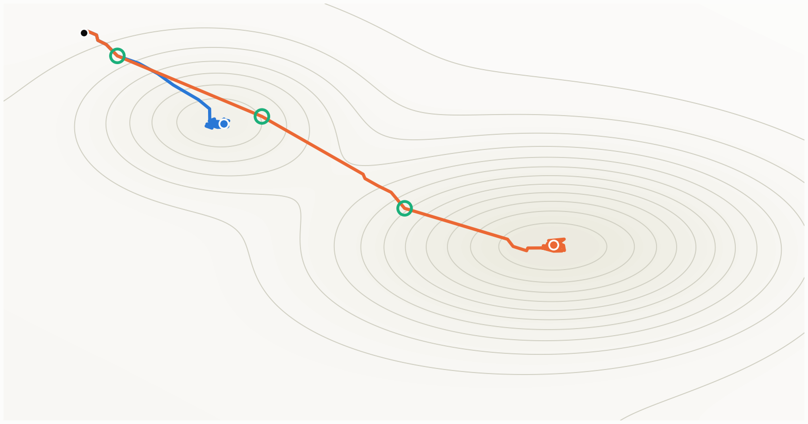
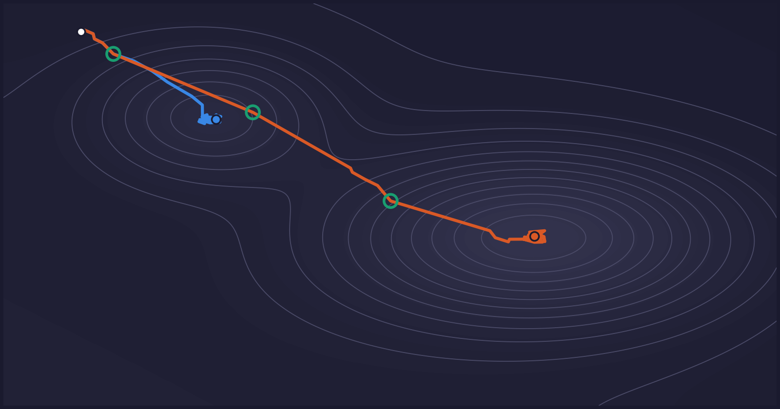
A two-basin cost landscape with an unsteered trajectory settling in a local minimum and a steered trajectory reaching the intended minimum.
Chat is how we drive AI agents now, and it feels entirely natural: give the model context, watch it work, drop in a correction when it drifts — “wrong layer, this belongs in the queue tier”, “you’re optimizing the 0.2%”. I steer coding agents like this all day, and a one-line correction at the right moment routinely saves an afternoon of confident, well-executed work in the wrong direction. What’s strange is how rarely we ask why this works. Steering is in-context learning: a few hundred tokens of text redirect a model whose weights never move. That it works at all is remarkable; that it works this well was, for me, a standing mystery. This post is my attempt to resolve it with theory.
The industry, meanwhile, has been naming its way up the same learning curve: prompt engineering, then context engineering, then harness engineering, now loop engineering — and lately even graph engineering? That ladder is the X in this post’s title: prompt, context, harness, loop, graph — pick your rung. Each coinage is honest engineers’ induction — a name for what practice discovered works — but induction without theory always sounds a little buzzy. My aim here is to supply the missing lines of thought: one foundation picture under which every rung becomes sound and sensible rather than fashionable.
The claim: an agent run is stochastic gradient descent (SGD) over solution space, and steering is how the true objective enters the loop. Two classic frames make the pattern legible — the cost landscape from optimization, and prior-to-posterior updating from Bayesian inference. Neither is offered as a proven mechanism of what happens inside the model; they are the lenses that make the observed behavior cohere, and where real theory backs a step, I cite it.
The question is no longer academic, either. Cursor recently published Agent swarms and the new model economics: a frontier model plans and delegates while fleets of cheaper models execute, and on their large benchmark task the stratified swarm cut the bill from $10,565 to $1,339 at comparable quality. That is steering as a product architecture — a big model guiding small ones through nothing but context. The frames in this post are one way to understand why that bet pays — and when it, rather than the classic alternative of teacher-student distillation, is the right tool for the work agents do daily.
An agent run is stochastic gradient descent
Map the pieces — with the contract stated up front: the descent here is over solution space, not weight space. The model’s weights never move during an agent run; what moves is the work-in-progress. Each agent step (read a file, run a test, write a patch) revises that artifact using whatever local signal the step produced, and the revision has the same form as the classic SGD update:
| SGD term | Agent-run counterpart |
|---|---|
| Parameters | The working artifact — architecture, framing, code |
| Loss | Distance from what the user actually wants |
| Gradient estimate | The feedback one step produces — test results, tool output |
| Learning rate | How much of the artifact one action may change |
In symbols:
where denotes the state of the working artifact after step — the architecture, the framing, the code so far; is the step size — how much of the artifact one action is allowed to change; is the agent’s proxy loss, its interpretation of what the user wants; and is the noisy gradient estimate, with collecting the per-step randomness from sampling temperature, tool outcomes, and retrieval luck.
In Eq. (1), the catch is the object being descended. The true loss — the distance between the artifact and what the user actually wants — appears nowhere in it, because is never directly observable; the agent can only descend its proxy . The noise term is harmless — SGD thrives on noise. The killer is bias — a systematic gap between and . A biased gradient doesn’t make the agent wander; it makes the agent converge, efficiently and confidently, to the minimum of the wrong function.
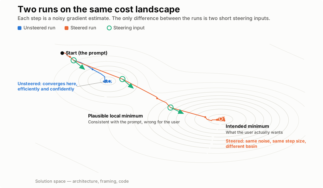
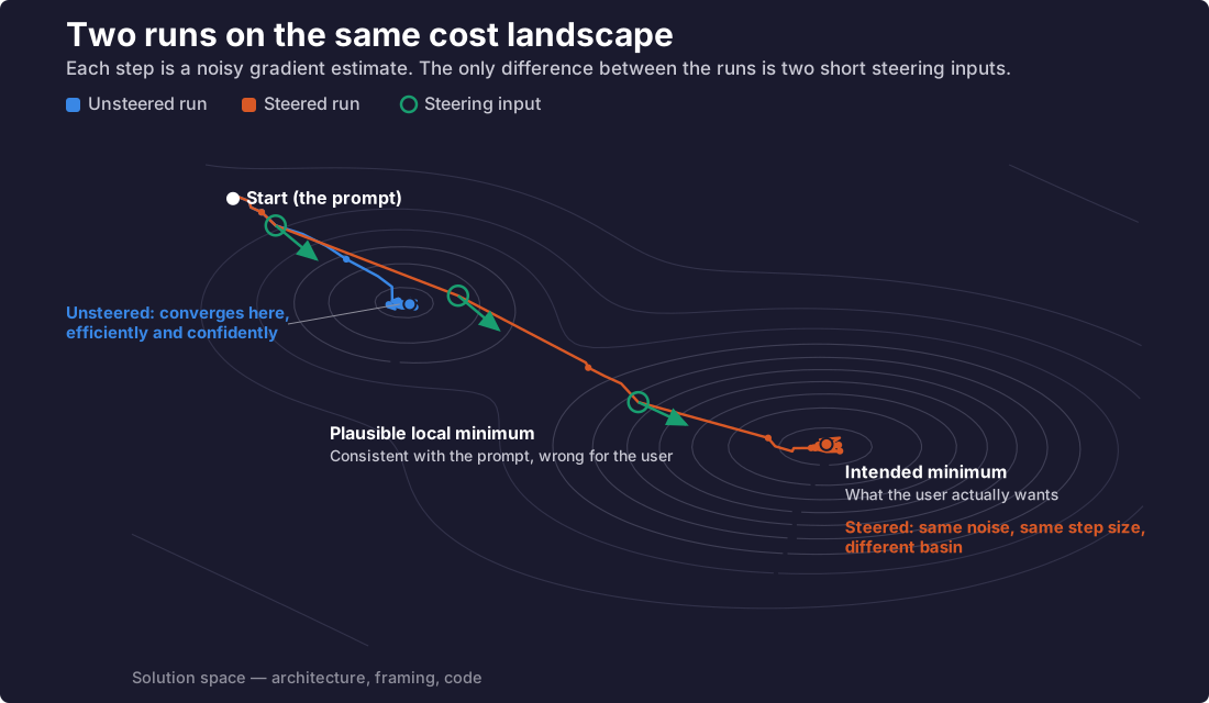
Fig. 1 is a simulation of exactly that. Both trajectories share the starting point (the prompt), the step size, and the noise sequence. The unsteered run falls into the nearer basin — a solution consistent with the prompt but wrong for the user — and settles. The steered run receives two small correction vectors early on and lands in the intended minimum. Nothing about the steered run is smarter; it just got fresh gradient information about the true loss at two moments where the proxy was about to commit to the wrong basin.
Two properties of steering fall out of this picture:
- Steering is a bias correction, not a productivity signal. The un-steered agent doesn’t stall — it produces plausible work at full speed. That’s precisely what makes the failure expensive: by the time the divergence is visible in the output, the trajectory has compounded hundreds of steps of drift. A correction at step 5 costs one sentence; the same correction at step 500 costs a rewrite.
- Large steering inputs are basin escapes. “This whole approach is wrong” is not a gradient nudge — it’s a momentum kick over the ridge. That’s why a hard redirect mid-session often works better than deleting the session: the accumulated descent still counts; only the direction was wrong.
One precision note before the analogy runs away: none of this happens inside the transformer. At inference the weights are frozen — decoding is a forward pass, and the KV (key–value) cache is memoization, not memory that learns. The only literal SGD in the life of a large language model (LLM) is training-time next-token prediction; the descent described here lives one level up, in the agent loop, where the loop itself is the optimizer.
That said, the analogy has a studied mechanistic spine. There are really three nested descent loops, and each outer loop builds the inner one:
- Weights — training. Literal SGD. But it doesn’t just learn a prior: autoregressive pretraining meta-learns an inference-time optimizer — mesa-optimization, internal optimization executed in the forward pass (von Oswald et al., 2023).
- Context — inference. In linear-attention settings, a forward pass over in-context examples provably implements gradient-descent steps, the update written into activations instead of parameters (von Oswald et al., 2023; Dai et al., 2023; contested for full-scale LLMs — Shen et al., 2023). The KV cache sits inside the fast-weights duality: for linear attention, appending a token is a rank-1 update to an implicit weight matrix (Schlag et al., 2021) — a lineage that test-time-training layers make literal by running actual SGD steps in the hidden state at inference (Sun et al., 2024).
- Artifact — the agent loop. The loop this post is about: the state is the work-in-progress, the gradient is feedback, and steering is the correction term.
Here is the part I find genuinely interesting: nobody trains the middle loop. No frontier lab runs a meta-learning algorithm — no model-agnostic meta-learning (MAML), no bi-level optimization; the recipes, where published, are ordinary SGD pretraining plus ordinary multi-turn reinforcement-learning (RL) post-training. An inner learner emerges — behaviorally certain, mechanistically still argued over — because across a broad enough task distribution the cheapest way to predict the next token is to become a learner, and the cheapest way to win multi-step tool-use episodes is to adapt mid-episode — read the failing test, revise the plan, try again. That is the classic RL² observation (Duan et al., 2016; Wang et al., 2016): train a policy across enough environments with in-episode feedback, and the learning algorithm migrates inward, executing in state rather than weights. Meta-learning is a property of the solution, not of the algorithm. And it explains something I feel every model generation: steering keeps getting more effective, because agentic post-training never teaches the model your task — it sharpens the very loop that steering feeds.
The frames also connect at the bottom, through an object worth defining rather than name-dropping: a Langevin process, the canonical noisy descent of statistical physics —
where is the state of the process; is an energy landscape — for training, the loss; for decoding, an energy such as negative log-probability; the drift term slides deterministically downhill; is Gaussian white noise (the increment of a Wiener process); and the temperature sets the size of the random kicks.
In Eq. (2), temperature decides what the process is. Run cold () and the noise vanishes: it is an optimizer, settling into the nearest minimum. Run warm () and it becomes a sampler: noise carries it over barriers, and at equilibrium it visits states with probability — the Boltzmann distribution, deep basins visited often, shallow ones rarely. The exponential is not an extra assumption: drift pumps probability into the wells while diffusion leaks it out toward sparser regions, and the Boltzmann density is the unique one at which the two fluxes cancel everywhere () — so the equilibrium is reached exactly when piling-up balances spreading-out. (Note: If equilibrium distributions are new territory, Appendix derives this chain step by step, from one particle to the exponential.)
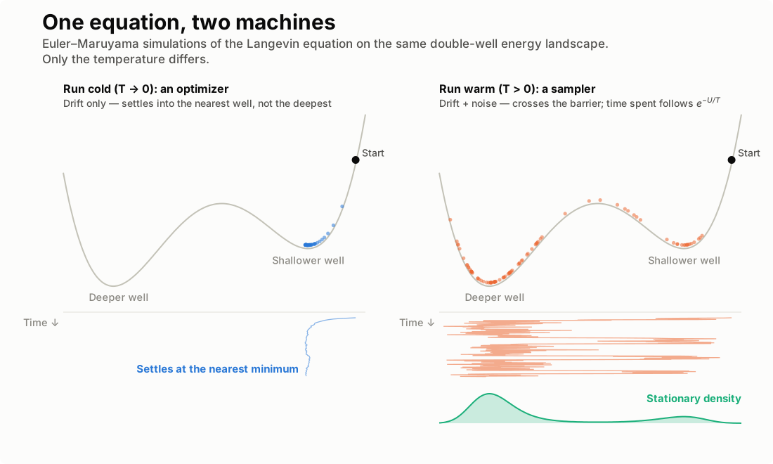
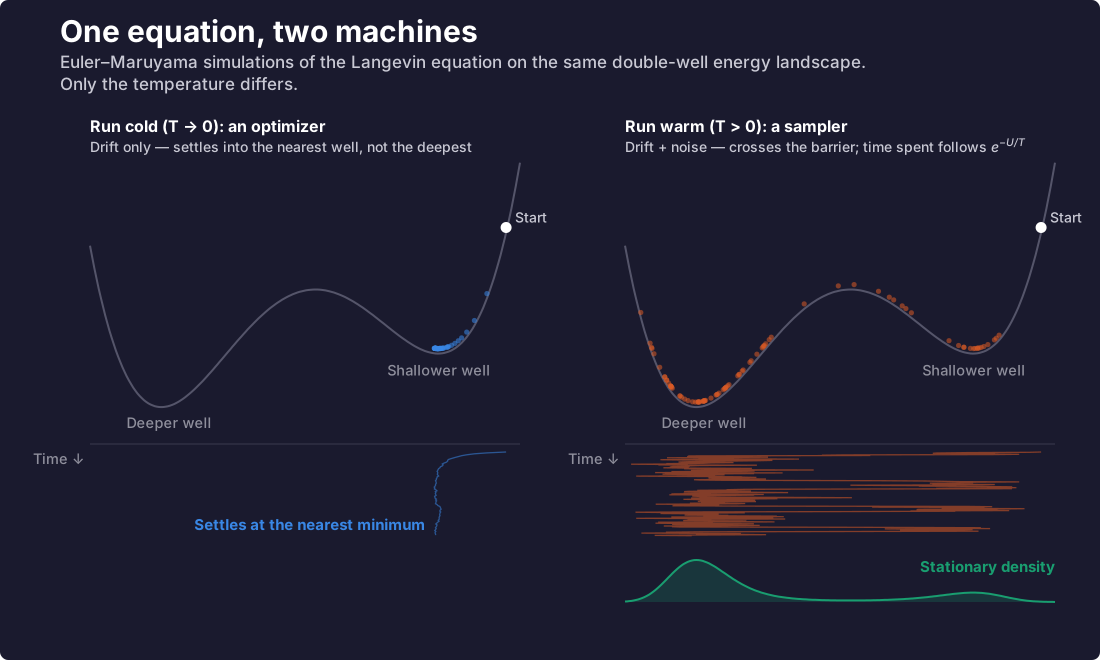
This is the bridge between the two frames of this post. SGD is Eq. (2) with drift from the gradient and noise from minibatching — which is why it can be read as approximate posterior sampling (Mandt et al., 2017) — and temperature- decoding samples from . Optimization and sampling are one process with the noise dial at different settings, and that is why the optimization view above and the Bayesian view below are the same fact twice.
The Bayesian crux: prior in the weights, posterior in the context
The landscape describes the search dynamics. The information dynamics are Bayesian, and they explain where the bias comes from.
At every step the agent holds an implicit belief about “what does the user want”, and that belief obeys Bayes’ rule:
where the prior lives in the weights — everything pre-training baked in about what code, designs, and answers usually look like; the evidence is the context window, so the likelihood scores how well a candidate intent explains the prompt, the tool results, and every steering message so far; and the posterior is the sharpening belief the agent acts on at each step.
In Eq. (3), the context is the only channel through which evidence reaches the agent — and here is the trap that makes steering necessary rather than optional: most of that context is written by the agent itself. Every token it generates joins the context and gets treated as evidence — but it’s evidence drawn from the prior, not from the world. An early wrong guess doesn’t fade; it hardens, each subsequent step conditioning on it more deeply. The posterior sharpens without ever touching ground truth.
The autoregressive machinery makes this trap structural, not incidental. During training, the model predicts each token conditioned on a ground-truth prefix (teacher forcing) — that’s where the literal SGD happens, and the conditioning prefix is always evidence from the world. At inference, the same machinery free-runs: each prefix token is the model’s own earlier sample, and the model was never trained on its own mistakes. That train/inference mismatch is the classic exposure bias problem (Ranzato et al., 2016), and its signature — small early errors compounding down the sequence — is the token-level miniature of everything this post describes at session scale. Seen this way, steering is the inference-time analogue of teacher forcing: it splices ground truth back into the prefix, at the only granularity available once the weights are frozen.
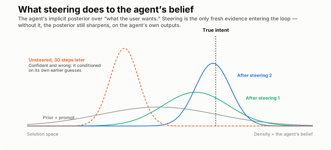
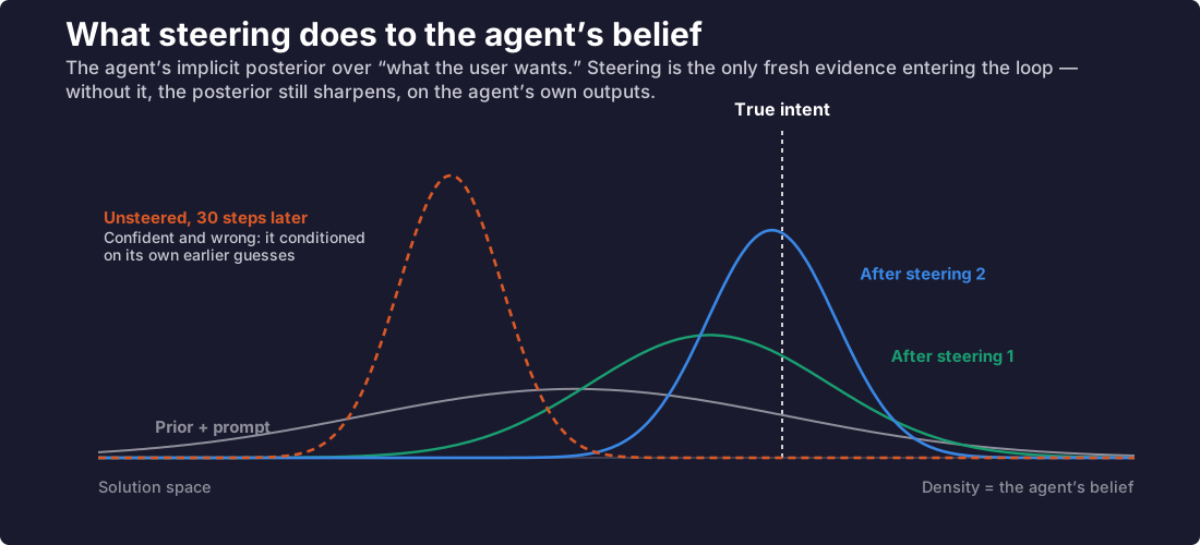
Fig. 3 shows both futures. With steering, each input is a likelihood term that shifts and sharpens the posterior toward the true intent. Without it, the posterior still sharpens — the dashed curve — but around the agent’s own earlier guesses: confident and wrong. Un-steered agents don’t fail by staying vague. They fail by becoming certain.
The two frames are the same fact viewed twice. A steering message is simultaneously a gradient correction (it re-aims the descent) and a Bayesian update (it injects the only evidence in the loop that came from outside the model). And this framing isn’t just an analogy of convenience: in-context learning behaving as implicit Bayesian inference is a studied result (Xie et al., 2022).
Why big models can steer small ones
If steering is evidence injection, the natural question is: whose evidence? Increasingly, the answer is another model’s. A support-desk triage
system shows the mechanism end to end. A classifier reads every incoming customer reply and makes two calls: which state the ticket should be in —
needs_agent or waiting_on_customer — and, for a message without a ticket reference, which open ticket it belongs to. The classifier is a local
open-source 35B mixture-of-experts model — ~3B active parameters, 4-bit quantized, thinking disabled for latency — and that model is the production
reality: no stronger variant is coming. Frontier models get exactly one role, offline diagnosis of the small model’s failures; they never see customer
traffic.
On a fourteen-trace golden eval, the small model was stuck at twelve, and the frontier coding agent running the eval had a ready diagnosis: capability wall — too few active parameters, quantization noise as large as the decision margins, no thinking budget. Its recommendation was to add code guards or swap in a stronger model. But that diagnosis rested entirely on comparing scores — frontier passes, local fails — so I pushed back with one steering message: don’t compare the scores, compare the reasoning — run both models on the failing traces and diff what they say, not what they conclude. The diff turned both “capability” failures into teachable ones:
- Gap 1 — the missed state flip. A support rep asks the customer to try reinstalling; the ticket is parked in
waiting_on_customer. The customer replies: “Tried the reinstall, same crash. What should I do now?” The ball is now with the support team, but the small model leaves the ticket parked — echoing the loudest string in the summary is cheaper than the inference we asked → they delivered → our move now. The frontier model’s reasoning opens with the signal the small model never mentions: “the reply comes from the customer (sender: customer) and ends in a question; the ticket cannot stay waiting on them.” The prompt, it turns out, taught only one direction — rep asks, park the ticket — never the mirror. Rule transferred: a customer who delivers what was asked and asks back flips the ticket toneeds_agent. - Gap 2 — the confident wrong merge. A message with no ticket reference: “Hi, the export is broken again since the update.” Two open tickets fit — CSV export timeouts (long, detailed history) and PDF export failing (two lines, opened yesterday). The spec says: two plausible matches and nothing in the message to decide → route to a human. The small model instead merges into the CSV ticket, citing “the customer references the timeout behavior” — words that exist only in that ticket, never in the message (Fig. 3’s dashed curve on a real trace). The frontier model names the trap outright: “a weaker model will prefer the candidate with the richer history, mistaking having more to say about a ticket for a better match to it.” Rule transferred: two plausible tickets with nothing in the message to decide means route to a human, never merge on a guess.
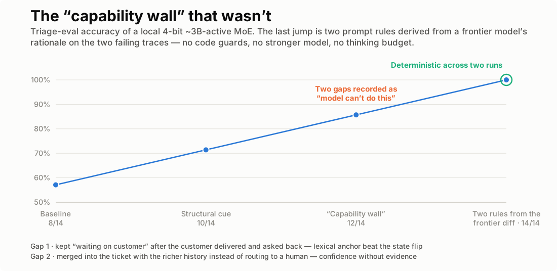
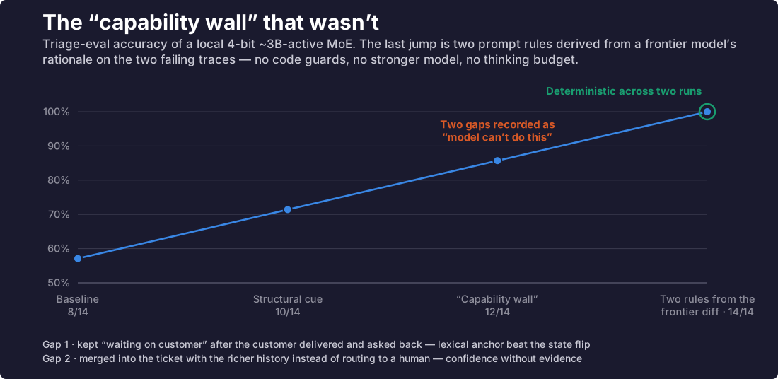
Those two sentences, written into the small model’s prompt, took the same quantized model to a perfect score, deterministic across two runs. No code guards, no stronger model, no thinking budget. Both frames say why the teacher’s rationale is the thing to transfer:
- Landscape: the student’s own prompt-space gradient is noisy — an earlier generic “route to a human when unsure” line had fixed one trace and broken another, because 4-bit decision margins are razor-thin. The teacher’s rationale is a low-noise gradient: it names the exact missing term of the objective, so the correction lands without collateral damage.
- Bayes: the teacher’s final answer (“route to a human”) is one bit and nearly useless; its rationale is the high-information evidence that, conditioned into the student’s prompt, moves the posterior for the whole class of cases. Gap 2 is a calibration failure — the student’s posterior collapses exactly where the teacher’s stays honest about ambiguity.
Note the nesting: a human steered the frontier agent (“compare the reasoning”), and the frontier agent’s reasoning steered the small model — the same mechanism, two levels deep. The economics rest on one asymmetry: judging a direction is much cheaper than walking it. The teacher read fourteen traces once, as an oracle; the student reads every customer reply, forever. Steering bandwidth is tiny compared to execution bandwidth — which is why one strong model can steer many cheap ones, and why one human can steer many agents. Cursor’s planner-and-workers economics from the introduction are this same asymmetry, monetized at fleet scale — and their model router prices it per request: route each step to the cheapest model that can take it, and frontier-level quality comes back 30–50% cheaper, because few steps genuinely need the model that supplies the judgment.
Distillation or in-context guidance?
The support-desk episode moved a small model with two sentences of context. The classic way to move a small model is the other lever entirely: teacher-student distillation. The three nested loops from the SGD section say exactly what the choice between them is — a teacher has two doors into a student, the weight loop and the context loop, and distillation takes the outer one. It is Eq. (1) run literally: are real parameters, the teacher’s outputs define the target, and the student gradient-descends toward it. It comes in two forms, one at each end of the training pipeline:
- Pre-training distillation matches distributions: the student trains against the teacher’s per-token soft probabilities instead of one-hot labels — Hinton’s original “dark knowledge” (Hinton et al., 2015). This is now standard for training strong small models: Gemma 2’s 9B and 2B were trained this way against a larger teacher, and NVIDIA’s Minitron line prunes then distills.
- Post-training distillation matches outputs: the teacher generates instruction responses or reasoning traces, and the student is fine-tuned on them — sequence-level rather than logit-level. DeepSeek-R1’s distilled Qwen and Llama variants are the best-known recent example, and virtually every synthetic-data pipeline is this in disguise.
Logit-level or trace-level, the edit lands in the same place: the weights. In the language of Eq. (3), distillation moves the prior — it changes what the student believes before any context arrives. Steering takes the inner door: no gradient ever fires, the teacher’s knowledge enters as conditioning text, and what moves is the posterior. Same knowledge transfer, transposed from weight space into context space — the same descent, one level up the loop stack.
How much is the outer door worth? In 2026 the market put a number on it. Anthropic disclosed coordinated distillation campaigns against Claude — over 16 million exchanges harvested through roughly 24,000 fraudulent accounts, attributed to DeepSeek, Moonshot, and MiniMax — with attackers specifically prompting the model to articulate its internal reasoning, because traces are the richest training signal. By July, Moonshot’s Kimi K3 was topping a blind coding arena while introducing itself as “Claude, an AI assistant made by Anthropic” in the wild; a widely-circulated community-compiled report compiles the broader allegations — benchmark contamination, arena routing, trace harvesting — which Moonshot denies. And the defense tells the same story as the attack: frontier vendors now return reasoning to API callers as encrypted thinking signatures rather than plaintext tokens, precisely so the chain of thought cannot be farmed — the report claims one lab broke the scheme and decrypted a billion reasoning tokens for about $60k. Why is the CoT specifically the thing to steal and the thing to encrypt? The support-desk story already said it: the final answer is one bit; the rationale is where the information lives. A reasoning trace is the teacher’s gradient written out in text — which makes it the crown jewel of trace-level distillation: valuable enough to harvest at scale, and valuable enough to lock.
The transposition is rarely a stylistic choice; often the inner door is the only one open. In the support-desk story the production model is a quantized third-party checkpoint — the weight loop simply isn’t there to run. And even when it is, moving the prior is an offline loop — collect data, train, evaluate, redeploy — that runs at training-pipeline cadence, days to weeks, and bakes in a snapshot of a task distribution. Steering inputs are the opposite in every dimension: per-task, arriving at conversation cadence, on a long tail — this classifier’s who-owes-the-next-move rule, this pipeline’s extraction format, this repo’s layering convention. No one distills a checkpoint per prompt rule. When the weights are frozen, the context is the only lever there is — and it turned out to be enough:
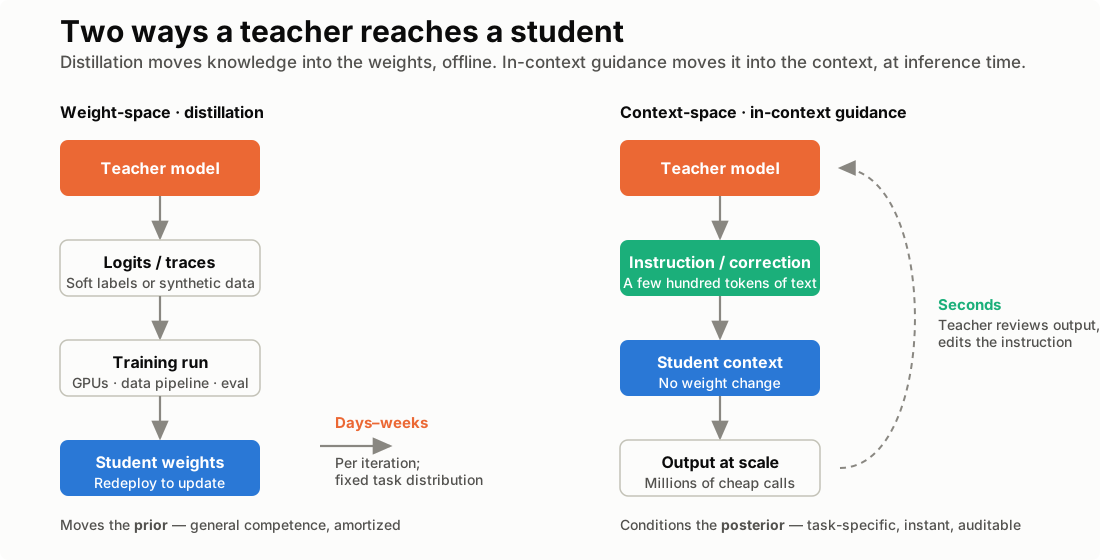
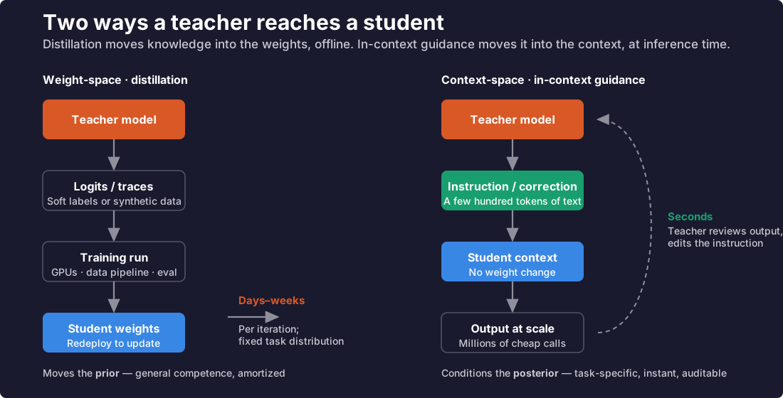
Zero-shot in-context guidance is distillation’s fast path: the teacher’s knowledge enters the student as a few hundred tokens of conditioning text instead of a weight update. The same knowledge transfer, but the iteration loop collapses from days to seconds — and the transferred artifact is text, so it’s auditable, editable, versioned, and reversible in a way weights never are. The triage fix is the concrete case: the entire transfer was two sentences derived from the teacher’s rationale, one of which over-fired, got diffed against a regression, and was tightened — all inside a single session. A distillation pipeline would still have been collecting traces.
To be fair to the outer door, the theft economics also mark out exactly when distillation is the right tool. Weight-space transfer is a high-fixed-cost, zero-marginal-cost channel: you pay for data and training once, and every future call benefits — no extra context tokens, no added latency, no prompt budget consumed. It also carries what text cannot: a soft distribution transfers calibration, style, and tacit skill — thousands of rules nobody knows how to state — which is why R1-distilled students jump in ways no instruction could deliver, and why sixteen million stolen traces are worth more than any prompt library. So the choice has a clean shape. Distillation wins when the task distribution is broad and stable, the volume is enormous, the weights are yours to train, and the capability is tacit. Steering wins when the weights are frozen, the tail is long, the task changes faster than a training loop can track, and the transfer must stay auditable. One is a factory; the other is a conversation — and the reason the factory owners have started locking up their traces is that the factory’s raw material turns out to be the same thing steering runs on: the teacher’s reasoning.
| Weight-space (distillation) | Context-space (in-context guidance) | |
|---|---|---|
| Update rule | A literal gradient step, Eq. (1) | A Bayesian update, Eq. (3) |
| What moves | The prior (weights) | The posterior (context) |
| Iteration cycle | Days–weeks | Seconds |
| Task scope | Fixed distribution, amortized | Per task, long tail |
| Infrastructure | Data + training + eval pipeline | None |
| Artifact | Opaque checkpoint | Readable, editable text |
| Marginal cost per task | A training run | A few hundred tokens |
The two mechanisms compose rather than compete. Distillation is why the small model can follow instructions at all — general competence, bought offline, amortized over everything. In-context guidance is the per-task specialization on top — the steering. Distillation builds the student; steering aims it.
The loop is the unit of engineering
The industry has started naming this picture. The discipline stack that began with prompt engineering and grew through context engineering has acquired two more layers: harness engineering — the environment a single agent runs in: tools, permissions, verification surfaces, memory — and, one level above it, loop engineering. Its most direct source is Boris Cherny, the creator of Claude Code, describing his own setup: self-verification loops are the ingredient that lets a powerful model run for long stretches and still land close to the intent.
The frames in this post say what that stack is, one line per layer. Prompt engineering chooses the starting point . Context and harness engineering shape the gradient — the tests, tools, and verification surfaces a step can draw on determine the quality of in Eq. (1). Loop engineering designs the optimizer itself: when the loop runs, which verifier injects the correction, where state persists between runs. The industry’s newest discipline is the recognition this post has been circling the whole time: the loop is the optimizer, and steering is a component you can engineer. A verifier subagent is a standing steering signal; a scheduled objective re-check is a periodic bias correction; persisted memory is the posterior, carried across sessions.
And the human doesn’t exit the picture — they move one loop out. When Cherny says “I don’t prompt Claude anymore. I have loops running that prompt Claude,” the steering that used to be typed turn-by-turn has been compiled into the loop, and his judgment now steers the loop’s design instead. That is the nesting from the support-desk story extended one level: the human steers the loop, the loop steers the agent, and the agent, sometimes, steers a smaller model still. Each level transmits judgment downward at a fraction of the bandwidth of the work it directs — which is, by this point in the post, exactly the asymmetry you should expect to find at every level. And the newest coinage, graph engineering — wiring many loops into an organization — is this same nesting drawn out as a diagram: more optimizers, more steering channels, the same asymmetry at every edge.
Lessons
Steer early, steer often. Bias compounds geometrically along a trajectory. The cheapest correction is the one delivered before the agent’s posterior sharpens around its own guess.
Watch for confident convergence, not for stalling. An agent in the wrong basin looks productive. The warning sign is certainty without external evidence. Gap 2 is the canonical tell: the model justified its choice by citing a detail that existed only in the ticket it picked, never in the customer’s message — when the stated reason quotes the conclusion instead of the input, the confidence came first and the evidence was invented after.
Diff the reasoning, not the answer. “Frontier passes, local fails” is a score, not a diagnosis. Comparing the two models’ rationales on the failing traces turned a “capability wall” into two named, promptable rules. When the oracle solves what the student can’t, its reasoning usually hands you the exact rule to transfer.
Spend big-model tokens on direction, small-model tokens on execution. Judging a direction is cheaper than walking it. The teacher ran fourteen traces once; the student runs every customer reply, forever.
Distill for competence, steer for the task. Weight-space transfer amortizes what every task needs; context-space transfer handles the long tail no training loop can track. If you’re choosing between them for day-to-day agent work, you’re usually choosing the fast loop.
Optimization needs a true objective; the agent only ever has a proxy. Steering is the mechanism that keeps the two aligned — a gradient correction in one frame, fresh evidence in the other, and a few hundred tokens either way. That asymmetry, judgment being cheap to transmit and expensive to recompute, is what makes the whole arrangement scale: one steering signal, millions of steps.
Appendix: deriving the Boltzmann distribution
The claim under Eq. (2) — that a warm Langevin process equilibrates to — leans on machinery the main text compresses into one sentence. The subtlety is a change of viewpoint: Eq. (2) describes one particle, while the Boltzmann distribution describes a population. Three levels of description connect them; the main text jumps from the first to the third, and this appendix walks the middle.
Step 1 — from one particle to a density. Eq. (2) generates a single random trajectory — one marble rolling and jittering across the landscape. Now release a million identical marbles, each obeying the same equation with independent noise. The individual paths stop being interesting; what matters is what fraction of the marbles sits near each . That fraction is the probability density — and it evolves deterministically even though every marble moves randomly.
Step 2 — what “equilibrium” means. Started from a uniform scatter, the density changes: drift piles marbles into the valleys, noise keeps spraying them outward. Eventually the density stops changing; that limit is the equilibrium distribution . Equilibrium does not mean the marbles stop — every one keeps wandering forever. It means the flows balance, like a busy train station at noon: individuals constantly in motion, yet reliably two hundred people near the entrance, five hundred on the platforms, a hundred in the café. The individuals move; the distribution doesn’t.
Step 3 — the equation the density obeys. Asking “how does evolve?” converts the Langevin equation into its population-level counterpart, the Fokker–Planck equation:
where is the drift flux — probability carried downhill by the gradient — and is the diffusive flux — probability leaking from dense regions toward sparse ones (Fick’s law), with the temperature setting the leak rate. Eq. (4) is to Eq. (2) what a crowd forecast is to one pedestrian: the same dynamics, tracked as a cloud instead of a point.
Where does Eq. (4) come from? Four moves: discretize, take moments, conserve, expand. (One-dimensional notation from here on, for readability; the vector form is identical with .)
(a) Discretize Eq. (2). Over a small step , the particle’s displacement is
where is the noise accumulated during the step — Gaussian with mean zero and variance . That variance is the defining property of Brownian noise: successive kicks are independent, and independent variances add, so variance grows linearly in time — which means the typical size of is . Keep that square root in view; it does all the work below.
(b) Take moments of . The mean is immediate — the noise averages to zero:
For the mean square, note that is a deterministic number plus a random term, so expands like any binomial and the expectation distributes across it by linearity (constants pass through an average untouched). The two facts needed are and — the latter because the mean square of a zero-mean variable is its variance: . Then:
Notice the asymmetry: the drift contributes to the mean at order but to the mean square only at order (negligible), while the noise contributes nothing to the mean but order to the mean square — because . The same square-root scaling kills every higher moment: , , all vanishing faster than . This is why exactly two moments survive — no more, no fewer.
(c) Write the conservation identity (Chapman–Kolmogorov). Now connect the density at two moments in time — using nothing but conservation of probability. A marble is near at if and only if it was somewhere at and its jump landed it at , so count every way that can happen. A marble that lands at after a jump of must have started at ; summing over all jump sizes:
where is the probability of a jump for a particle currently at . Read it as a ledger: the fraction near now is the sum, over all origins, of the fraction that was there times the chance of jumping here — every marble accounted for, none created or lost. Two things make this step trustworthy. First, it is exact: pure conservation of probability, nothing approximated — the approximation enters only in (d). Second, it relies on exactly one assumption: the process is Markov, meaning memoryless — the jump distribution depends only on where the particle is, not on how it got there. Eq. (2) guarantees this: the drift is a function of the current position alone, and each noise kick is independent of every previous one, so a particle’s history adds no information about its next move. This composition rule — the distribution later equals the distribution now composed with the transition probabilities — is precisely what the Chapman–Kolmogorov equation says; the name refers to the ledger identity itself, not to any additional mathematics.
(d) Taylor-expand and integrate. The integrand depends on twice — as the jump size, and through the starting point . Bundle the starting-point dependence into one function, , and Taylor-expand it in its first argument around :
Now integrate over term by term. The -derivatives don’t involve , so they pull out of each integral — and each remaining integral collapses into a moment. Why: with the first argument fixed at , we have , and contains no — it is a constant of the integration and factors out. What is left, , is the average of weighted by its probabilities — the definition of , the -th moment. So (a probability density integrates to one: the particle certainly jumps by some amount, with counting as a jump), , and . (This is also why the expansion was taken around at all: its entire purpose is to move the -dependence out of ‘s argument so the integrals factor.) Therefore
Substitute the moments from (b) — first moment into the first-derivative term, second moment into the second-derivative term, everything higher vanishes:
Subtract , divide by , let , and restore vector notation: Eq. (4), exactly. In words: the mean jump becomes advection, the mean-square jump becomes diffusion. Langevin and Fokker–Planck are not two laws — they are one law read at two zoom levels, converted by averaging over the noise and keeping the two moments that survive.
Step 4 — impose equilibrium. At equilibrium nothing changes, so : the net flow out of every region vanishes. In equilibrium the stronger statement holds — the probability current itself vanishes everywhere, not merely its divergence (in a confining landscape with no probability escaping at the boundaries, a divergence-free current must be zero):
which is exactly the flux-balance condition quoted in the main text: downhill pumping cancels outward leaking, pointwise.
Step 5 — solve it. Divide Eq. (5) by and recognize a logarithm:
where is an integration constant. Exponentiating both sides turns the additive constant into a multiplicative one:
where is the normalization constant that makes the density integrate to one. The famous exponential is not an assumption — it is the unique stationary, zero-current solution of Eq. (4).
The three levels, side by side:
| Level | Object | Governing equation |
|---|---|---|
| Microscopic | One particle’s position | Langevin, Eq. (2) |
| Mesoscopic | The density | Fokker–Planck, Eq. (4) |
| Macroscopic | The stationary density | Boltzmann, Eq. (6) |
The middle row is where the two frames of this post become one object: Eq. (4) is simultaneously the flow of an optimizer’s iterates and the update of a sampler’s belief. Drift is the gradient step, diffusion is the exploration, and which machine you are looking at depends only on the temperature.