Collection Autofill at Scale
May 28, 2026
A design walkthrough of how Collection Autofill — a spreadsheet of AI-computed cells — stays fast, fair, and observable from a hundred rows to ten million.
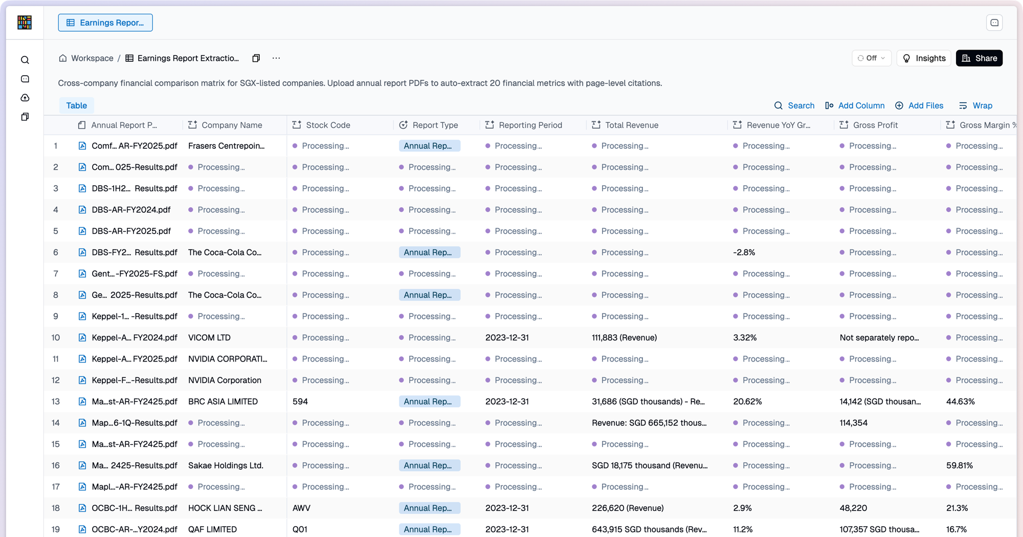
An Instill AI Collection mid-autofill, every cell processing.
Imagine a spreadsheet where any cell can be AI-computed: a URL column, an AI-generated summary that depends on it, an AI-generated sentiment that depends on the summary. Edit one URL, and a small DAG of cells recomputes. Now imagine you have ten million such cells, and a single user just clicked Reprocess column.
That’s the design problem behind Collection Autofill — a feature in Instill AI that lets users define AI-computed cells and watch them recompute automatically. This post is a walkthrough of how it works at scale: the contract we promise users, the architecture that makes it true, the handful of design calls that ended up doing most of the work, and why we leaned on Temporal, Postgres, and Redis instead of the alternatives.
A note on Collections
A bit of product context first. Collections are the core pillar of Instill AI — the surface where unstructured data becomes structured context. The inputs aren’t only static uploads (documents, images, videos, audio): they include dynamic sources too — a web URL the system fetches and re-fetches, an RSS feed, a connector pulling rows from another system. Each input becomes a row; AI-generated columns extract, summarise, classify, or otherwise derive each row into queryable fields. A folder of contracts becomes a table you can filter by counterparty, expiry, and risk; a list of competitor URLs becomes a market-watch sheet that re-grades when pages change; a library of meeting recordings becomes a table you can search by topic and decision; a research corpus — files, links, and live feeds intermixed — becomes a knowledge base your downstream agents can reason over. A Collection is what turns “a folder of stuff and a stack of links” into “a database I can ask questions of”.
That’s also why we don’t think of Collections as “AI spreadsheets” alone. That product choice reflects a few deeper architecture bets:
- The table is the natural interface for cross-source work — when data comes from many places and the job is comparison, extraction, correction, and state tracking, a table is closer to how people actually work than chat or search.
- Trust has to be enforced by schema and execution — if a cell should not be guessed, that cannot live only in the prompt. The column definition, cell state, and UI all need a way to represent “there is not enough evidence” instead of letting the model force an answer.
- The same primitive serves extraction and generation — when organizing data, Collection compresses scattered context into reliable fields; when generating content, the same fields and DAG constrain style, role, and factual consistency. The use case is different, but the underlying engine is the same.
- Knowledge work is becoming multi-modal on both sides — documents, images, videos, audio, URLs, and feeds all become inputs; outputs will not stay text-only. Collection needs to be the shared interface that can carry those modalities.
So the Collection product concept rests on four pillars:
- Structured context — Collections turn files, URLs, live feeds, recordings, and other unstructured inputs into queryable fields.
- Static and dynamic sources — inputs can be uploaded once, fetched repeatedly, or synced from another system as rows change.
- Column-defined workflow DAG — AI-generated columns can depend on other columns, so the table schema itself defines the recomputation graph.
- Human and agent interoperability — users can inspect, correct, override, and monitor the data, while agents rely on the same structured state for reasoning and downstream actions. The two views must stay connected and observable instead of becoming separate systems.
Autofill is the engine that fills those AI-computed cells, regardless of whether the input was a static file or a live URL. It’s the bridge between whatever raw context you pointed the system at and the structured context the system surfaces — which means it has to be fast, fair, and observable at any scale a real user might throw at it.
That makes Autofill’s execution design rest on a different set of pillars: transactional queue correctness, bounded durable orchestration, stateless and idempotent cell compute, fairness and isolation, latest-write safety, and separate scaling axes for setup orchestration and cell computation.
What we’re actually building
A Collection in Instill AI is a tabular structure (i.e., spreadsheet) with one twist: columns can define computation, not just storage. Any column can be configured as AI-computed, and AI-computed columns can depend on other columns. That column dependency graph is the workflow DAG Autofill has to execute. Edit a URL in column A and column B’s AI summary recomputes. Mark column C’s sentiment as depending on B’s summary, and editing the URL fans out: A → B → C. Multiply by ten thousand rows and the schema-level DAG becomes a large cell-level recomputation graph.
The contract is deceptively simple to describe and quite hard to implement well. Each AI cell carries two values — what you typed and what the AI produced; user input always wins for display. The system has to handle: per-collection fairness so one big reprocess can’t starve everyone else, per-namespace in-flight caps so one tenant can’t monopolize the worker pool, latest-write safety under overlapping recomputes, schedule modes (compute on change, never, or on a cron), file inputs that arrive asynchronously, and a UI that wants live progress updates. That’s the bar.
Why a naïve Temporal-only design doesn’t scale
The natural first attempt is to put everything in Temporal: one workflow per row, per-cell activities awaited inside the workflow’s selector. Conceptually clean — one workflow per scope, an activity record for each cell, durable execution end to end. It’s the design any engineer with Temporal experience would prototype first.
flowchart TD
  T([Recompute trigger]) --> W([Temporal workflow])
  W -->|"Schedule one activity per cell<br/>(all awaited in a single selector)"| A([Per-cell Temporal activities])
It works beautifully at the demo scale of a hundred rows. Above 50,000 cells, four things compound.
1. The selector loop becomes single-threaded. Every per-cell future is awaited inside one workflow’s selector. Temporal’s selector is fast, but it processes futures one at a time. At a million cells, scheduling overhead alone consumes roughly a hundred seconds before the first LLM token comes back. The workflow looks busy; nothing observable is happening.
2. Temporal history grows linearly with cells. Each per-cell activity writes two history events; a million-cell run produces two million. That’s well past Temporal’s 10,240-event soft warning (the threshold at which it nudges you to call Continue-As-New) and on track for its 51,200-event hard cap, where the server terminates the workflow. There’s a parallel 50 MB total-history-blob limit too.
3. There is no per-collection fairness. One greedy bulk reprocess on collection A consumes every available LLM-queue slot in the cluster — a user editing a single cell on collection B waits until A’s bulk run finishes, sometimes hours later. The dispatch loop has no notion of “this is a different tenant; let it cut the line”.
4. Setup and cell-compute deploy together. Both live in one binary, but they change at very different cadences: prompts and tool wrappers get tweaked several times a week; the workflow lifecycle (shared-cache build, completion-aggregation tick) is touched once a quarter. Coupled deploys mean every prompt change is also an orchestration restart — dropping in-flight cache leases and blinking SSE streams. They scale differently too — cell-compute by LLM throughput, orchestration by active-collection count — but the shared binary forces one shape onto both.
The first two are about Temporal being asked to do the wrong job. It’s a brilliant tool for orchestrating workflows with bounded numbers of events —
for processes that need durable state, retries, signals, and human-readable history. It is not a queue. The moment you write
for cell in 1..N { schedule activity }, you’ve built a queue on top of Temporal’s history mechanism, and you’ll pay for it twice — once in
scheduling overhead, once in storage. The third and fourth aren’t Temporal’s fault; they follow from putting cell-level scheduling and per-collection
orchestration in the same place.
The architecture
Sit with the constraints and they suggest their own answer.
- Cell-level work is stateless and idempotent. Workers just need to claim a cell, run an LLM call, write the result. If a worker dies, another picks it up. That’s a queue, not a workflow.
- Per-collection orchestration is a workflow. Building a shared cache (DAG, credit check, namespace), aggregating completions, emitting batched progress events, recording usage — all of that benefits from durable execution and bounded history.
- The two have different deploy cadences. They should be separate binaries.
So Collection Autofill has three components and one singleton, separated along exactly those seams.
flowchart TD
  SR["Signal reconciler<br/>(service-layer dispatch)"]
  PG[("Postgres queue<br/>autofill_state column")]
  WP["Cell-worker pool<br/>(stateless · no Temporal)"]
  RS[("Redis Stream<br/>autofill:completions:*")]
  SW["Setup workflow<br/>(one Temporal workflow per active collection)"]
  J["Janitor<br/>(Temporal singleton · 30 s tick)"]

  SR -->|UPSERT 'queued'| PG
  SR -->|SignalWithStart| SW
  PG -->|claim batch| WP
  WP -->|finalize| PG
  WP -->|publish completion| RS
  RS -->|periodic drain| SW
  SW -->|batched progress + usage| Client([client])
  J -->|reclaim stuck · retry transient| PG
In one sentence each:
- Signal reconciler — a service-layer dispatch primitive every trigger surface goes through. It atomically queues cells in Postgres and signals the per-collection workflow.
- Setup workflow — exactly one Temporal workflow per active collection. Owns the bounded orchestration: shared cache, completion aggregation, progress emission, usage recording. Calls Continue-As-New on idle, so its history never grows linearly with cell count.
- Cell-worker pool — stateless pods, no Temporal client. Each worker grabs the next un-claimed work item from the Postgres queue using
SELECT FOR UPDATE SKIP LOCKED(a Postgres pattern where many workers race for rows without blocking each other — locked rows are silently skipped instead of queued behind), runs the LLM call, and writes the result back with a guard that commits only if no one else has touched the cell since the claim (a compare-and-swap; a slow worker that got reclaimed can never overwrite a fresher one). Completion events go on a Redis Stream for the setup workflow to drain. - Janitor — a Temporal singleton that reclaims stuck cells and retries transient failures on a 30-second tick. The platform enforces “exactly one” via the workflow ID; no per-pod leader election needed.
That’s it for the topology.
Three decisions that did most of the work
The architecture above is the obvious half. The non-obvious half is three smaller decisions that paid for themselves daily.
Separate state columns, not overloaded ones
The cell row carries two state machines in distinct columns:
- Cell-status state (user-visible): “is the AI’s answer ready”, “is it outdated”, “is the spinner showing”, “what failed”, and the actual value. This is what the frontend reads.
- Queue state (worker-internal): an
idle / queued / computing / done / errorenum, a queued-at timestamp, a dirty flag for overlap handling. This is what the worker pool reads.
The two never share columns. Three repository methods (upsert, claim, finalize) are the only places that touch both, and each does so in one atomic SQL statement with the sync rules baked in.
A naïve design overloads shared columns to mean different things at different lifecycle points. Half the race conditions in this kind of system live in those overloads. Splitting the state spaces and gating the bridge through three atomic methods retires entire classes of bugs — without changing a single line of frontend code. The user-visible contract is invariant; only the implementation underneath it changes.
If I had to name one decision I underestimated going in, this is it.
Dirty flag over cancellation
What if a cell is mid-LLM-call and the user reprocesses it again? The naïve answer is “cancel the in-flight call and start over”. That answer is wrong twice over: you’ve already paid for the in-flight call (LLM tokens aren’t refundable), and “cancellation that cleans up correctly” is a notorious source of bugs.
The better answer is a dirty flag. When a new signal arrives for a cell already computing, we record a “fresher signal arrived” timestamp on the cell
and let the in-flight call finish. At finalize time, the worker checks: if a fresher signal came in since this attempt started, the queue state goes
back to queued after the attempt instead of settling as terminal. The next claim cycle picks it up; the user gets a fresh recompute. Cap the loop at
three rounds so a pathological signal storm can’t burn money forever.
flowchart TD
  Q([Queued]) -->|Worker claim| C([Computing])
  C -->|"Finalize · clean<br/>(or attempts cap reached)"| D([Done])
  C -.->|"Finalize · dirty flag set<br/>(re-queue · attempts++)"| Q
Dirty flags shift the guarantee from “cancel obsolete work” to “obsolete work cannot win”. That is the right guarantee for LLM-backed cell computation: retries, reclaims, and dirty requeues can run the work again, but the visible cell converges to the latest signal, and the compare-and-swap guard prevents an old claim from overwriting a fresher one. Three states and three edges express the entire dirty-flag mechanic; the rest of the state machine (cancel signals, janitor reclaim, transient retries) hangs off this same state model.
Two binaries, decoupled
The deployment topology is the cheapest part of the design and pays back daily. Setup orchestration and cell computation run as separate binaries — one with a Temporal client, one without — because they have fundamentally different roles, scaling characteristics, and resource profiles.
The setup-worker binary owns the per-collection setup workflow plus the cluster-wide janitor. Its job is coordination: build the shared cache (DAG, namespace, credit lookup), drain the Redis-Stream completion bus, batch progress notifications to the frontend, record token usage, reclaim stuck cells, retry transient failures. It scales modestly — bounded by the number of active collections (a few dozen at any moment), not by the number of cells — and carries the heavyweight initialisation for gRPC clients to Redis, the metrics pipeline, the storage layer, and the management backend.
The cell-worker binary is a pure goroutine pool — twenty goroutines per pod by default — that runs a tight claim → LLM call → finalise loop. Each goroutine atomically claims work from Postgres at the grain the queue shape calls for (cell, row, or batchable column), sends a gRPC request to the Python LLM worker, writes the result back, and publishes a completion event. There’s no Temporal client, no workflow registration, no task-queue polling. Just a DB connection, an LLM-worker gRPC client, and a Redis publisher. Scaling is linear in cells-to-process: ten pods × twenty goroutines = two hundred concurrent LLM calls.
Four reasons that decomposition matters:
Independent scaling axes. Cell-workers are CPU- and network-bound (waiting on LLM calls) and you want many of them — one per claimed work item in flight. Setup-workers are IO-bound coordinators and one or two replicas suffice. In a single binary you’d either over-provision Temporal pollers when scaling for LLM throughput, or under-provision cell-workers when scaling for collection count. Two binaries let each side scale to its own bottleneck.
Failure isolation. A cell-worker crash mid-LLM-call strands only the cells that pod claimed — they sit in Computing until the janitor (in the setup-worker) reclaims them. If both responsibilities lived in the same process, a crash would take out the worker and its own recovery mechanism in one stroke.
Different restart semantics. The setup-worker leans on Temporal’s durable execution — workflows survive restarts via event replay. The cell-worker is stateless and disposable: kill it, restart it, scale it to zero, and the Postgres state machine is the only thing that matters. Mixing workflow-style replay with a stateless goroutine pool in one binary complicates shutdown ordering and graceful drain.
Different resource profiles. Cell-workers are network-bound and need many goroutines; setup-workers are memory-bound (workflow replay history) and need a high concurrent-workflow-task ceiling but few goroutines. Different tuning, different pod resource requests, different horizontal-pod-autoscaler thresholds. One binary means one shape — and you’d tune it for the louder of the two concerns at the cost of the other.
Two operational concerns; two binaries.
Why Temporal, Postgres, and Redis — and not the alternatives
A reasonable reader will ask: did you really need three pieces of infrastructure? Couldn’t a single workflow engine, message bus, or stream-processing framework have done it all? Three short answers, one per layer.
Temporal earns its keep as the orchestration tier because the setup workflow needs durable state, signals, and Continue-As-New: it has to survive deploys, coalesce overlapping triggers, hold a 5-minute Redis cache lease, and emit batched progress ticks for as long as a collection is active. That is a workflow, not a job. A DAG scheduler like Airflow assumes batch runs on a calendar; a task queue like Celery has no first-class signals or durable workflow state. Temporal is exactly the right shape — the rebuild’s lesson is only that it’s the wrong shape for the cell-dispatch tier inside it.
Postgres earns its keep as the queue tier for one decisive reason: the queue state and the cell value need to be transactionally consistent. When a worker finalizes a cell, “the queue says this work is done” and “the cell row shows the AI result” must succeed or fail together. With Postgres that’s one transaction; with a separate queue product like Kafka, NATS, or SQS it’s two systems and a distributed-commit problem, plus a separate rate-limiter to recover the fairness that a SQL window function gives us directly (cap each collection, and optionally each namespace, to N in-flight claims). When your work items already live in a relational database and your retries are crash-safe, Postgres-as-queue is hard to beat.
Redis earns its keep as the in-flight messaging bus because the ask fits its shape exactly: small completion envelopes for the setup workflow, ephemeral progress frames for the UI, and shared-cache invalidation markers between workers. Kafka would be over-engineered (per-topic cost doesn’t amortise; we don’t need long-lived analytical retention); Pulsar or NATS add a fourth stateful system to save twenty milliseconds. Redis was already in the stack for shared cache; making it carry the bus cost nothing extra.
One last cross-cutting alternative worth naming: someone with a data-engineering background will reasonably ask whether this should have been a Flink or Kafka Streams job — events in, events out. The answer is no for three reasons. The workload is bursty rather than continuously streaming; the cells are independent transforms with no windows or joins; and a stream processor’s checkpoint-and-state-backend overhead is enormous relative to “claim a row, finalize a row”. Stream processors are the right answer for real-time aggregations, multi-stream joins, time-windowed metrics. They are not the right answer for a per-cell idempotent LLM transform fed by a queue.
The temptation in any greenfield design is to reach for one shiny piece of infrastructure that solves everything. The discipline is to notice that you have three layers with three different requirements — durable orchestration, transactional queue, transient messaging — and let each one pick its tool independently.
At scale
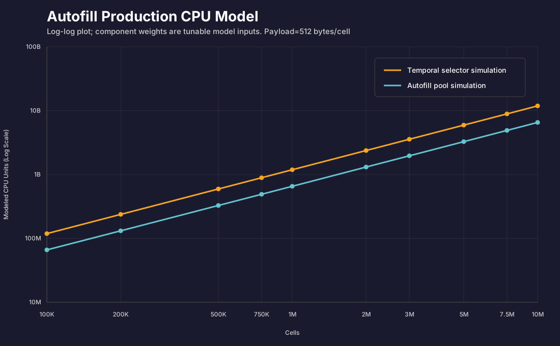
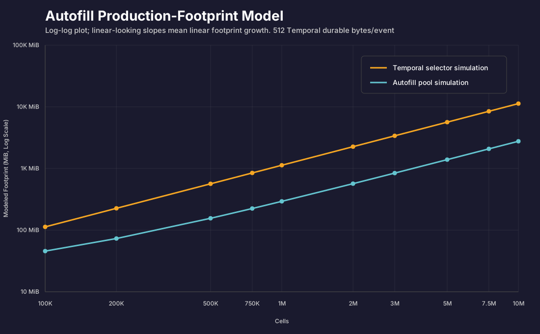
To sanity-check the 100K-10M-cell design target, I added a small in-process benchmark for the scheduling/state-machine layer. It allocates cell state, runs concurrent claim/finalize workers, measures real CPU work, and models production CPU plus memory/storage footprint by component. The run below used 200 workers, 16 collections, 4 namespaces, two Temporal events per cell, 512 durable bytes per Temporal event, 512 serialized payload bytes per cell operation, 192 row bytes plus 96 index bytes per pool queue cell, and no dirty requeues. It is still not a claim that a production deployment processed ten million live cells in one run.
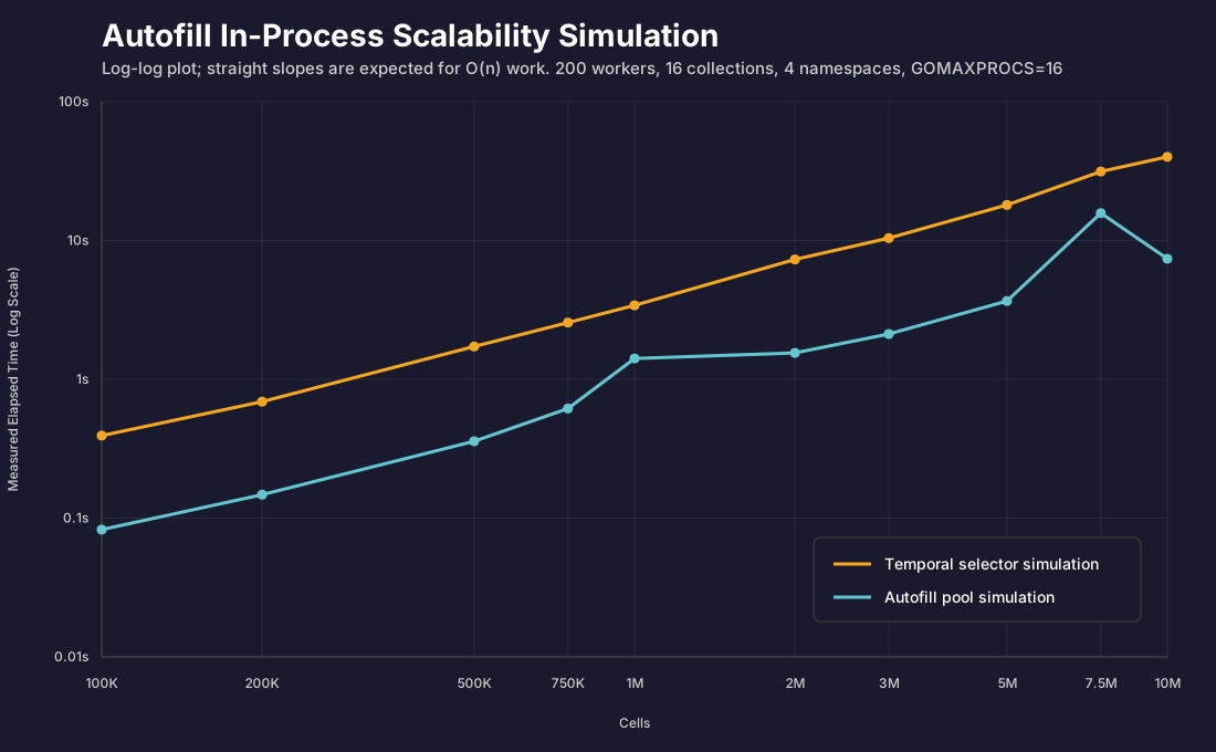
The chart uses log-log axes, so a nearly straight line is expected for an O(n) workload. The useful signal is that both designs scale roughly linearly with cell count in this simulation, while the worker-pool architecture has a lower constant factor and avoids the Temporal history event growth that makes the naïve design operationally invalid long before ten million cells.
| Naïve Temporal-only | Collection Autofill | |
|---|---|---|
| 1M-cell simulator elapsed time | ~ 3.41 s | ~ 1.41 s |
| 1M-cell simulator throughput | ~ 293K cells/s | ~ 708K cells/s |
| 1M modeled CPU units | ~ 1.19B | ~ 655M |
| 1M modeled app heap pressure | ~ 153 MiB | ~ 13.3 MiB |
| 1M modeled total footprint | ~ 1.13 GiB | ~ 293 MiB |
| Temporal history events | ~ 2,000,000 per run | ≤ 10,000 per Continue-As-New window |
| Per-cell Temporal activity records | One per cell | Zero |
| Per-collection fairness | None | Per-collection cap, SQL-enforced |
| Per-namespace in-flight fairness | In-memory, single-process | SQL-enforced when the cap is enabled |
| Backpressure observability | Indirect | One SQL query against the queue table |
| Setup vs cell-compute deploy coupling | One binary | Two binaries, independently scalable |
The user-facing contract is preserved end-to-end. Reset, Reprocess, Schedule modes, undo/redo, the spinner, the progress hover — all unchanged. The frontend doesn’t need to know any of the above exists.
Where this design starts to bend (the 10B horizon)
The current architecture’s design target is the 100K–10M-cell range per collection, with the bottleneck shifting from orchestration overhead to LLM throughput, queue-claim contention, and completion aggregation. The next walls — partitioned column workflows for very wide columns, dedicated task queues per collection, true batch LLM inference, per-cell version vectors so we don’t recompute cells whose upstream values haven’t changed, hash-partitioning the cell table at very large scale — are all written down. None are urgent. They all come from the same question: at the next order of magnitude, where does this design break first?
Lessons
A few patterns worth tattooing on a younger version of the team.
Use Temporal for what it’s good at — bounded orchestration with durable state, retries, signals, and human-readable history. Not millions of
events. The moment you find yourself writing for x in 1..N { schedule activity }, you’ve built a queue on top of a workflow engine and you’ll pay
for it forever.
Postgres is a perfectly good queue for stateless retry-safe work. SELECT FOR UPDATE SKIP LOCKED plus window-function fairness caps gives you
per-collection and per-namespace budgeting in SQL — observable, queryable, indexed. It’s been in Postgres since 9.5 and it’s still the right answer
when your work items are idempotent.
Separate state columns beat overloaded ones. If two state machines live in the same row, give them two distinct sets of columns and gate the bridge through a small number of atomic methods. The cost is a few extra columns; the payback is that nobody ever again has to reason about what a single “started” timestamp means here vs there.
Dirty flags beat cancellation. Cancelling expensive in-flight calls (LLM, external APIs, big queries) to honour a fresher signal wastes money and adds bug-prone cleanup paths. A dirty flag plus a cheap re-queue gives latest-signal convergence with simpler code.
Symmetric API surfaces age well. When every variant of a verb (cell, row, column × single, batch) funnels through the same dispatch primitive, adding a new axis later doesn’t fork the dispatch logic. It’s also much easier to get right once.
Two binaries are not over-engineering. When the dominant operational cost and the coordination cost change at different cadences, separate binaries pay back the day you do your first capacity rollout without touching the orchestration tier.
Architectures are a story of which forces you decide are first-class. Collection Autofill makes three: the queue must be transactionally consistent with the cell value, orchestration must be durable but bounded, and worker compute must be stateless and idempotent. Three forces, three layers, three different tools — Temporal, Postgres, Redis — each picked because nothing else cleared the bar for its layer. That’s the trade you want.
Onwards to ten billion cells.